Communications cables are, by design or necessity, often installed in proximity and/or in the same pathway as power service cables. The electrical energy of the power cables can have a significant effect on the performance and safety of these cables. It is very important to ensure that electromagnetic interference (EMI), or dangerous levels of electrical energy are not induced into telecommunication cables.
This paper discusses the effects of the terrain and parameters that could influence the field in high-voltage power lines and communication cables. Power transmitting towers are usually 10m to 40m high and the separation between two consecutive towers is about 200m to 400m. Finite Element Method (FEM) is not suitable for simulation in these applications. BEM is useful on very large domains where a FEM approximation would have too many elements to be practical. Integrated Engineering Software’s COULOMB’s BEM solver is best suited to simulate this problem. It is based on a boundary integral equation, which allows the unbounded problem to be entirely defined at its boundary and therefore reduces the number of variables required to solve it. This methodology can be used to find the potential gradients not only over the surface of the conductors but also anywhere of interest in space.
https://www.integratedsoft.com/
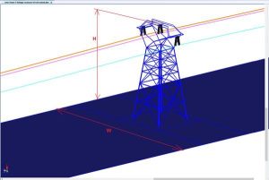
Figure 1
W as the width of the ground plane and H as the height of the tower, the following cases were considered.
(a) W=H, for analyzing the electric field on the ground and 1 meter above the ground.
(b) W=3H, for analyzing the field in the space between the power lines and 1 meter above the ground.
It should be noted that the number of 2D triangular elements on the ground will increase as the size of the ground plane increases and the solver will take a longer time. This time can be reduced if lower (1/100) triangular element density (number of triangular elements per unit area) is taken as compared to the element density on the insulator strings and metallic hardware. Electric field analysis for W=H and W=3H (see Figures 2a and 2b) showed that there is not much difference between E-field variations for both cases. So, the W=H case is considered a good case to analyze the problem as it could reduce problem complexity and produce highly accurate results.

Figure 2 a
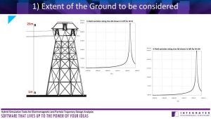
Figure 2b
Figure 3 shows a power line setup with 200-400m separation between two towers. If power line is considered as a thin long cylinder with a radius of 1cm to 3 cm, then it would require a vast number of 2D triangular discretization elements, and the model would not be easy to solve. To simplify this, power lines could be assumed as linear segments which would need 1D discretizing elements.


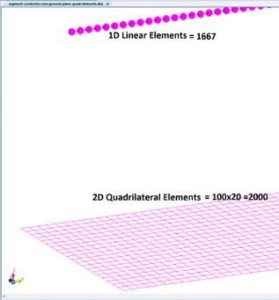
Figure 3
For comparison, both cases (linear segments and thin cylinder power lines) were analyzed. Figure 4 shows the plot of E-Field along the Line AB for both cases. It shows that results for linear segments overlap the plot for thin cylindrical power lines showing less than a 1% difference between both results. Hence, the simulation of power lines as linear segments is recommended to reduce the number of elements and faster solution.
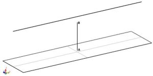

Figure 4
Keeping the desired sag in overhead power lines is an important consideration, hence while calculating the fields at the communication cable, sagging in the cable should also be simulated. If the amount of sag is very low, the conductor is exposed to a higher mechanical tension which may break the conductor. Whereas, if the amount of sag is very high, the conductor may swing at higher amplitudes due to the wind and may contact alongside conductors. For equal heights of the towers, maximum sag S = u *L*L/(8T), where u is the weight per unit length of the power line, L is the span length, T is the optimum mechanical tension applied to the line. The shape of the sagged line is very close to a parabola. Usually, the parameters u and T are not readily available, but the maxim sag S is. Figure 5 shows the E-field plot along the communication line. It is seen that the field near the points A&B is significantly higher than that in the middle point C.
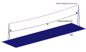

Figure 5
It can take a lot of time to simulate a transmission tower due to the complexity of the model. Hence, it is better to model only the part of the tower where the insulation strings are connected to the power lines, approximating the rest of the tower as a solid structure. Both cases were simulated to see the difference. Figure 6 shows electric field plots for actual tower geometry and for part of the geometry with communication lines only. It is seen that plots of both cases overlapped and hence simulating the part of the tower could produce accurate results while saving a lot of time.
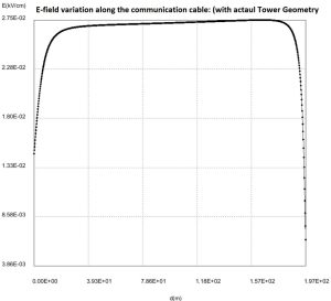


Figure 6
